Example 4: Two-dimensional convection and diffusion

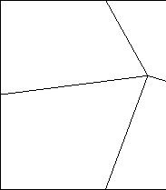
This example demonstrates the effect of the spatial stabilization algorithm in 2D. A convection and diffusion of heat equation is analyzed on a 1 by 1 square. The two-dimensional mesh consists of distorted linear quadrilaterals

The convection velocity $\beta=1$ and the conductivity $k=0.01$. The boundary conditions for temperature are chosen such that the exact solution for a boundary layer in $y$-direction holds:

$$T(y) = T(y=0) + (T(y=1)-T(y=0)) \frac{1- \exp (\beta\frac{y}{k})}{1-exp(\frac{\beta}{k})}$$

where we choose $T(y=0)=1$ and $T(y=1)=0$. This is a severe test for the spatial stabilization algorithm. Many algorithms exist which solve this example exactly when using a one-dimensional domain, say with $y$-axis only, but few exist which do not show wiggles for irregular 2D grids. The node_dof records are initialized with temperature 1 as a first estimate for the solution field. The we check the results at $x=0.7$ and $y=0.6$. The exact solution is 1. The numerical solution with the 4-noded elements is 0.95. Splitting the elements in triangles (see control_mesh_split) would have given the solution 1.001. Triangles seem to behave better than distorted quads (in this example anyway). Both solutions are quite good however.