Hypo-Plasticity

In hypoplasticity a direct relation is used between strain rates and stress rates. Specifically:

$$\dot{\sigma}_{ij} = L_{ijkl} \dot{\epsilon}_{ij} + N_{ij} \sqrt{ \dot{\epsilon}_{kl} \dot{\epsilon}_{kl} }$$

Here the part with $L_{ijkl}$ gives a linear relation between strain rates and stress rates and the part with $N_{ij}$ gives a nonlinear relation. The constitutive tensors $L_{ijkl}$ and $N_{ij}$ are functions of the effective stress tensor $\sigma_{ij}$ and void ratio $e$. The effective stress tensor $\sigma_{ij}$ follows from the total stress tensor $\sigma_{ij}$ minus any pore pressures (see groundflow). Rigid body rotations (objectivity) are treated elsewhere (see the section on memory).

Basic law, Wolffersdorff

The law proposed by WOLFFERSDORFF [11] is used.

$$\begin{eqnarray*} & L_{ijkl} = f_s \displaystyle \frac{1}{\hat{\sigma}_{mn}\hat{... ...[ \hat{\sigma}^*_{mn}\hat{\sigma}^*_{mn} \right]^{3/2}} \quad .& \end{eqnarray*}$$

For $\hat{\sigma}^*_{ij}=0$ is $F=1$.

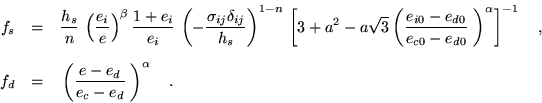
The scalar factors $f_s$ and $f_d$ take into account the influence of mean pressure and density:

$$\begin{eqnarray*} f_s &=& \displaystyle \frac{h_s}{n}\,\left(\displaystyle \frac... ...t(\displaystyle \frac{e-e_d}{e_c-e_d}\;\right)^{\alpha} \quad . \end{eqnarray*}$$

Three characteristic void ratios - $e_i$ (during isotropic compression at the minimum density), $e_c$ (critical void ratio) and $e_d$ (maximum density) - decrease with mean stress:

$$\displaystyle \frac{e_i}{e_{i0}} = \frac{e_c}{e_{c0}} = \fra... ...- \left(-\frac{\sigma_{ij}\delta_{ij}}{h_s} \right)^n \right]$$

The range of admissible void ratios is limited by $e_i$ and $e_d$. The model parameters can be found in Tab. 1. They correspond to Hochstetten sand from the vicinity of Karlsruhe, Germany [11].

Table 1: Basic hypoplastic parameters of Hochstetten sand.

$\varphi$ [$^{\circ}$]	$h_s$ [MPa]	$n$	$e_{c0}$	$e_{d0}$	$e_{i0}$	$\alpha$	$\beta$
33	1000	0.25	0.95	0.55	1.05	0.25	1.0

The basic law parameters should be specified in group_materi_plasti_hypo_wolffersdorff.

Cohesion

A simplistic appraoch to include cohesion is used here. Instead of feeding the real effective stress state $\sigma_{ij}$ into the hypoplastic law, an alternative effective stress state $\sigma_{ij}^c$ is used. Cohesion is modelled by subtracting in each of the normal stress components a value $c$ representing cohesion: $\sigma_{11}^c = \sigma_{11} - c$, $\sigma_{22}^c = \sigma_{22} - c$ and $\sigma_{33}^c = \sigma_{33} - c$. The shear stresses are not altered: $\sigma_{12}^c = \sigma_{12}$, etc.

The cohesion value should be specified in group_materi_plasti_hypo_cohesion.

Intergranular strains

In order to take into account the recent deformation history, an additional tensorial state variable $S_{ij}$¹ is introduced.

Denoting the normalized magnitude of $S_{ij}$

$$\rho = \displaystyle \frac{\sqrt{S_{ij}S_{ij}}}{R}$$

(R is a material parameter) and the direction of $S_{ij}$

$$\hat{S}_{ij} = \displaystyle \frac{S_{ij}}{\sqrt{S_{kl}S_{kl}}}$$

( $\hat{S}_{ij}=0$ for $S_{ij}=0$), the evolution equation for the intergranular strain tensor reads:

$$\dot{S}_{ij} = \left\{ \begin{array}{lll} ( I_{ijkl}-\rho^{... ...ij}\dot{\epsilon}_{ij} \leq 0 \\ \end{array} \right. \quad ,$$

where $\dot{S}_{ij}$ is the objective rate of intergranular strain. Rigid body rotations are treated elsewhere (see the section on memory). From the evolution equation (2.2.4) it follows that $\rho$ must remain between 0 and 1.

The general stress-strain relation is now written as

$$\dot{\sigma}_{ij} = M_{ijkl}\dot{\epsilon}_{kl} \quad .$$

The fourth order tensor $M_{ijkl}$ represents the incremental stiffness and is calculated from the hypoplastic tensors $L_{ijkl}$ and $N_{ij}$ which may be modified by scalar multipliers $m_T$ and $m_R$, depending on $\rho$ and on the product $\hat{S}_{ij}\dot{\epsilon}_{ij}$:

$$\begin{eqnarray*} M_{ijkl} &=& [ \rho^{\chi} m_T + (1-\rho^{\chi})m_R ] L_{ijkl}... ...\hat{S}_{ij}\dot{\epsilon}_{ij} \leq 0 \\ \end{array} \right. \end{eqnarray*}$$

$\chi$ is an additional material parameter.

An example intergranular parameters can be found in Tab. 2.

Table 2: Example of Intergranular hypoplastic parameters.

$R$	$m_R$	$m_T$	$\beta _r$	$\chi$
$1\cdot 10^{-4}$	5.0	2.0	0.50	6.0

The intergranular parameters should be specified in group_materi_plasti_hypo_intergranularstrain. Also you need to include materi_strain_intergranular in the initialisation part.

Pressure dependent initial void ratio

You can correct the initial void ratio $e_{0}$, as specified in the initial value for the history variable in the node_dof records, for the initial pressure to obtain a corrected initial void ratio $e$.

$$\frac{e}{e_{0}} = \exp \left[ - \left(-\frac{\sigma_{ij}\delta_{ij}}{h_s} \right)^n \right]$$

See the basic law description for the parameters $h_s$ and $n$. The $\sigma_{ij}$ denotes the effective stress tensor (total stresses minus any groundflow pressure). This pressure dependent initial void ratio correction can be activated by group_materi_plasti_hypo_pressuredependentvoidratio. After the initial void ratio has been established, the development of the void ratio is governed by volumetric compression or extension of the granular skeleton.